
Tools for Molecular Systematics
Usefull scripts
Extract features from NCBI/GenBank annotation
The code below extracts nucleotide sequences from *.gb files and outputs the CDS found in fasta format.
extract_CDS.py
#
## Script modified from https://www.biostars.org/p/230441/
# This script extract CDS nucleotide sequences from mitochondrial refseq genomes
#	usage: python extract_CDS.py input_file.gb output_file.fas
#
from Bio import SeqIO
import sys

with open(sys.argv[2], 'w') as nfh:
        for rec in SeqIO.parse(sys.argv[1], "genbank"):
                if rec.features:
                        for feature in rec.features:
                                if feature.type == "CDS":
                                        nfh.write(">%s from %s\n%s\n" % (
                                        feature.qualifiers['gene'][0],
                                        rec.name,
                                        feature.location.extract(rec).seq))
The code below extracts aminoacids sequences of CDS from *.gb files and outputs the CDS found in fasta format.
extract_CDSaa.py
#
## Script modified from https://www.biostars.org/p/230441/
# This script extract CDS sequences of aminoacids from mitochondrial refseq genomes
#	usage: python extract_CDSaa.py input_file.gb output_file.fas
#
from Bio import SeqIO
import sys

with open(sys.argv[2], 'w') as ofh:
        for seq_record in SeqIO.parse(sys.argv[1], 'genbank'):
                for seq_feature in seq_record.features:
                        if seq_feature.type=="CDS":
                                assert len(seq_feature.qualifiers['translation'])==1
                                ofh.write(">%s from %s\n%s\n" % (
                                seq_feature.qualifiers['gene'][0],
                                seq_record.name,
                                seq_feature.qualifiers['translation'][0]))
The code below extracts tRNA sequences from *.gb files and outputs the tRNA sequences found in fasta format.
extract_tRNA.py
#
## Script modified from https://www.biostars.org/p/230441/
# This script extract tRNA sequences from mitochondrial refseq genomes
#	usage: python extract_tRNA.py input_file.gb output_file.fas
#
from Bio import SeqIO
import sys

with open(sys.argv[2], 'w') as nfh:
        for rec in SeqIO.parse(sys.argv[1], "genbank"):
                if rec.features:
                        for feature in rec.features:
                                if feature.type == "tRNA":
                                        nfh.write(">%s from %s\n%s\n" % (
                                        feature.qualifiers['product'][0],
                                        rec.name,
                                        feature.location.extract(rec).seq))
The code below extracts rRNA sequences from *.gb files and outputs the rRNA sequences found in fasta format.
extract_rRNA.py
#
## Script modified from https://www.biostars.org/p/230441/
# This script extract rRNA sequences from mitochondrial refseq genomes
#	usage: python extract_rDNA.py input_file.gb output_file.fas
#
from Bio import SeqIO
import sys

with open(sys.argv[2], 'w') as nfh:
        for rec in SeqIO.parse(sys.argv[1], "genbank"):
                if rec.features:
                        for feature in rec.features:
                                if feature.type == "rRNA":
                                        nfh.write(">%s from %s\n%s\n" % (
                                        feature.qualifiers['product'][0],
                                        rec.name,
                                        feature.location.extract(rec).seq))
As the script requires individual files, you can automate sequencial runs by using the following script:
for file in *.gb ; do python extract_*.py ${file} ${file%.*}.fas ; done
This code extracts individual genomes from concatenated genomes in GenBank (*.gb) format.
get_individual_genomes.pl
#!/usr/bin/perl
#
# usage:
#	perl  get_individual_genomes.pl input_file.gb
#
#
$file = $ARGV[0];
open (FILE, $file);
 while (<FILE>) {
   if ($_ =~ m/^LOCUS\s+(\w+).*/){
	$output_file = "$1\.gb";
	open($out, '>', $output_file);
	print $out "$_";
   }
   if (($_ =~ m/^[\w|\s|\d].*/) ne ($_ =~ m/^LOCUS.*/)){
	print $out "$_";
   }
   if ($_ =~ m/^\/\/\n/){
	print $out "$_";
	close ($out);
   }
 }
close (FILE);
Sequence submission to the NCBI/GenBank
Here I will provide some information on how to submit sequences to NCBI/GenBank using Sequin. It is the goal of this tutorial to make sure we standardize the information we associate with the sequences. This is important because not all the sequences deposited at NCBI for our group provide the same information (i.e, host data, voucher; among others) and even if they do, they are not in a standard format - that is, under the same source modifier (see bellow).
The information associated with sequences in the NCBI/GenBank is done by Source Modifier. The list of source modifiers provided by the NCBI/GenBank is long and among those we think that we should use at least these: Organism, specimen-voucher, isolate, dev_stage host, collected-by, collection-date, country, lat_lon, and note.
Table of modifiers
The first thing you have to build is a table with the following content:
| SeqId | Organism | specimen-voucher | isolate | dev_stage | host | collected-by | collection-date | country | lat_lon | note |
|---|---|---|---|---|---|---|---|---|---|---|
| Pararhin_EC_14.1 | Pararhinebothroides hobergi | MZUSP 7754 | EC-14.1 | adults | Urobatis tumbesensis | J. N. Caira & F. Marques | 24-May-2014 | Ecuador | S 2.19967, W 80.9780 | Host field number EC-14 |
| Pararhin_EC_56.1 | Pararhinebothroides hobergi | MZUSP 7755 | EC-56.1 | adults | Urobatis tumbesensis | J. N. Caira & F. Marques | 3-Jun-2014 | Ecuador | S 2.19967, W 80.9780 | Host field number EC-56 |
| Pararhin_EC_56.2 | Pararhinebothroides hobergi | MZUSP 7756 | EC-56.2 | adults | Urobatis tumbesensis | J. N. Caira & F. Marques | 3-Jun-2014 | Ecuador | S 2.19967, W 80.9780 | Host field number EC-56 |
| Pararhin_EC_56.3 | Pararhinebothroides hobergi | MZUSP 7757 | EC-56.3 | adults | Urobatis tumbesensis | J. N. Caira & F. Marques | 3-Jun-2014 | Ecuador | S 2.19967, W 80.9780 | Host field number EC-56 |
Here, the first row contains the source modifiers. The Sequence ID (SeqId) is the name of your sequence in the FASTA file. Thus remember, it is mandatory that the first column name matches the name of your sequences in the FASTA file. The other columns are pretty intuitive, but I should comment some modifiers. The isolate should receive your molecular code. The date of collection (date) has to be in the format: DD-month-YYYY (i.e., “24-May-2014”). The latitude and longitude data (lat_lon) should be inserted in a “semi-decimal” format (i.e., “S 2.19967, W 80.9780”). I say “semi-decimal” format because in LAT/LONG in an decimal format uses +/- for N/S and E/W, respectively. If your georeference data is in Degrees, Minutes, Seconds format, you can covert using Montana State University webpage. Finally, the host field number should be inserted under the source modifiers note, as in “Host field number XXXX”.
You can build this table in any spreadsheet application, but you will have to save that as a TAB delimited text file. You can download the table above in a TAB delimited format here.
Running Sequin
Once you have your table built, you can run Sequin. I will go through all the steps of Sequin using the sequence FASTA file below, which I will call example.fas. It is important to degap your sequences, that is, you should always submit unaligned nucleotide sequences.
>Pararhin_EC_14.1
ACAGGATGAGCCAGGATTCGCTCGGACACGATGGGCACGAGATTAGGACACAG
>Pararhin_EC_56.1
ACAGGATGAGCCAGGATTCGCTCGGACACGATGGGCACGAGATTAGGACACAG
>Pararhin_EC_56.2
ACAGGATGAGCCAGGATTCGCTCGGACACGATGGGCACGAGATTAGGACACAG
>Pararhin_EC_56.3
ACAGGATGAGCCAGGATTCGCTCGGACACGATGGGCACGAGATTAGGACACAG
So, as expected, the first thing to do is to open Sequin. You should get the following window:

In this window, you should click on “Start New Submission”. If you have already done one and want to use some of your data from the previous record (i.e., address, affiliation, among other) you can click on “Read Existing Record”. Regardless of your choice, you should get the following window:

Here you will insert all the information concerning the publication to which your sequences will be related, your contact, authorship, and affiliation information.

Note: In the window above, I selected the option in which I define the date in which the data should be public. By default, NCBI will give you one year. But you can make it longer or shorter as well as you can change the status of you sequence at any time by contacting the NCBI personal.
This step is pretty intuitive, after filling up all the fields in “Contact”, “Authors”, and “Affiliation” just click on the button “next page”. By doing so, you will obtain:

In this example, I am submitting a rDNA 28S sequence. Thus, I chose the option accordingly. Press “Next” and you will get the following window:

This is the window that allows you to import your External FASTA file. If you click on “Import Nucleotide FASTA”, you will get the option to choose the file you want to import (Remember: your file must have unaligned sequences!):

If all went well, you should get a summary of your imported sequences:

In this window, you will also have to provide the methodology you used to obtain your sequences under the tab “Sequencing Method”:

Here I selected sanger sequencing and indicated the they are “raw sequence reads”.
The next window will ask you the type of submission you are about to do. In this particular case, I want to associate the sequences with a phylogenetic study. Therefore, here is the option I selected:

Go to the next window.
Here, Sequin will ask from which organism you got your sequences. As you can see, there is no option for worms! Thus, I selected “something else”!

Move on to the next:

Here is an important step, since you will now use the table with the source modifiers you did as the first part of this tutorial. You should click on “import source table” and select the file. Once accomplished this step, go to the next window.

This window will ask you from which genome you obtained your sequences. Since we are submitting sequences of rDNA 28S, I selected Nuclear genome. Once you selected an option, go to the next.

Now you will have to select the type of fragment or genomic region you sequenced. In that case, I selected “single rRNA or ITS”. Move to the next.

Because I selected “single rRNA or ITS”, this window will ask some more details about my sequences. Select accordingly. In this case, I selected the option for rDNA 28S. Once you are done, go to the next:

Now you are basically done! You should select “Open Record Viewer”, because you will need to verify whether there are errors in your data and you will have to save the file to be sent to NCBI.
When you press “Open Record Viewer”, if no errors are found and reported, you should get the following:

Note: If you got an error message, please see the section on Error Reports below.
By default, the record viewer shows only the first sequence of your file. You could inspect one by one, to make sure all the information you desired is associated with your sequence. To finally export the file to be submitted to NCBI, you should select “ALL SEQUENCES” in “Target sequences” and click on “Done”.

Sequin will then ask if you want to save the record. Press “Yes”, and you will be presented with the following window:

Here you should give a name to the file and press “Save”.
Congratulations! You are done! Well, in part. Sequin finished its job, which was to generate a file compatible to the input files NCBI receive the sequences. After you saved the file, you will get the following warning message:

Pay attention to that! Here is the email to which you should send the file Sequin just generated. So, I guess, your job will be done once you email the file!
Error Reports in Sequin
According to NCBI, “[t]here are four types of error messages, Info, Warning, Error, and Reject. Info is the least severe, and Reject is the most severe. You may submit the record even if it does contain errors. However, we encourage you to fix as many problems as possible. Note that some messages may be merely suggestions, not discrepancies. A possible Warning message is that a splice site does not match the consensus. This may be a legitimate result, but you may wish to recheck the sequence. A possible Error message is that the conceptual translation of the sequence that you supplied does not encode an open reading frame. In this case, you should check that you translated the sequence in the correct reading frame. A possible Reject message is that you neglected to include the name of the organism from which the sequence was derived. The name of the organism is absolutely required for a database entry. If Sequin does not detect any problems with the format of your record, you will see a message that “Validation test succeeded”.
If you got an error message and was able to identify the error, you can reopen Sequin, start a new submission, but instead of following all the steps we discuss above, you select “Click here to import a template”. See figure below:

After importing the data, follow the steps of the program, which were discussed above. Good luck!
Tree editing and manipulation
Below I will give you some tips on how to deal with file manipulation during your phylogenetic analysis in order to avoid a lot of editing of file. As a rule of thumb, I like to keep the name of my terminals short and without characters that are bound to give you troubles as you migrate files from one application to the other (i.e., ”-“, ”&“, ”#“, among others). Underscore (i.e., “_”) is your only option most of the time.
Consider the following example of data file:
>Potamotrygonodestus_fitzgeraldae_amazon_PA03-53.1
ATTTACTATCATTCACATATCAAGAATGATGACAGATGAGCATGAC...
>Potamotrygonodestus_fitzgeraldae_amazon_PA03-53.2
ATTTATTAACATACACATATCAAGAATGATGACAGATGAGCATGAC...
>Potamotrygonodestus_marajoara_amazon_PA03-13.1
ATTTATTAACATACACATATCAAGAATGATGACAGATGAGCATGAC...
>Potamotrygonodestus_marajoara_amazon_PA03-13.2
ATTTATTAACATACACATATCAAGAATGATGATTTTTGAGCATTTC...
...
This format, encompasses the name of the species, its distribution and a code for the specimen sequenced. Some programs, and TNT is an example, would truncate names like this to 32 characters. Therefore, these programs would consider each of these taxon names as:
>Potamotrygonodestus_fitzgeraldae
ATTTACTATCATTCACATATCAAGAATGATGACAGATGAGCATGAC...
>Potamotrygonodestus_fitzgeraldae
ATTTATTAACATACACATATCAAGAATGATGACAGATGAGCATGAC...
>Potamotrygonodestus_marajoara_am
ATTTATTAACATACACATATCAAGAATGATGACAGATGAGCATGAC...
>Potamotrygonodestus_marajoara_am
ATTTATTAACATACACATATCAAGAATGATGATTTTTGAGCATTTC
...
Note that the two initial taxa would have the same name, the same is true for the last two, and that would be enough impede you to analyze this data.
I am aware we give names that would allow us to recognize the taxa as fast as possible. That I will try to convince you is that you can keep code names in your input files and use a simple tool to make the translations required whenever you need to visually examine the result of your analysis.
Here is how I would deal with that:
Usually, I use a code for each specimen. If I am dealing with hundreds of terminal, I use few letters and at least three digits. For instance, for the example above I would have something like:
>Pot001
ATTTACTATCATTCACATATCAAGAATGATGACAGATGAGCATGAC...
>Pot002
ATTTATTAACATACACATATCAAGAATGATGACAGATGAGCATGAC...
>Pot003
ATTTATTAACATACACATATCAAGAATGATGACAGATGAGCATGAC...
>Pot004
ATTTATTAACATACACATATCAAGAATGATGATTTTTGAGCATTTC...
...
Those taxon names will never give you a hard time in any application I am aware of! But of course, you need to keep track of what those codes means and most of the time, we do that by having a spreadsheet that document all our specimens or terminals. Let us then consider a two column table:
| Code | Specimen |
|---|---|
| Pot001 | Potamotrygonodestus_fitzgeraldae_amazon_PA03-53.1 |
| Pot002 | Potamotrygonodestus_fitzgeraldae_amazon_PA03-53.2 |
| Pot003 | Potamotrygonodestus_marajoara_amazon_PA03-13.1 |
| Pot004 | Potamotrygonodestus_marajoara_amazon_PA03-13.2 |
From this table, you can generate a text file called rename.sed in the following format:
s/Pot001/Potamotrygonodestus_fitzgeraldae_amazon_PA03_53_1/
s/Pot002/Potamotrygonodestus_fitzgeraldae_amazon_PA03_53_2/
s/Pot003/Potamotrygonodestus_marajoara_amazon_PA03_13_1/
s/Pot004/Potamotrygonodestus_marajoara_amazon_PA03_13_2/
This is a file formatted for Sed; a stream editor native to UNIX/LINUX systems, therefore also available in your Mac. Sed is a powerful toll when it comes to make substitutions in text files - remember, most of the files we manipulate during phylogenetic analyses are text files! Note: I did avoid to use ”-“ and ”.“, because depending on what you want to do, those characters will not work!
Here it how you can apply this tool. Consider that you for a tree output file, which we will call example.tre, with the following content:
(Pot003:0.00000,Pot004:0.04311,(Pot002:0.00000,Pot001:0.07118)0.98:0.09396);
Now, if you open a terminal window, move to the directory in which your files are, and execute the following command line:
sed -f rename.sed example.tre
You will get:

However, you may desire to redirect the output of the commmand line above to a file so that you can open the file in something like FigTree. In that case, you should execute the following command line:
sed -f rename.sed example.tre > example_renamed.tre
In this command line, the option ”-f“ of sed implied that all rules of substitution are in a file (i.e., rename.sed) and that the file to be translated is example.tre and the output of this sed command line should be redirected (the sign ”>“ is what does it) to the file example_renamed.tre. The content of the file example_renamed.tre should be:
(Potamotrygonodestus_marajoara_amazon_PA03_13_1:0.00000,Potamotrygonodestus_marajoara_amazon_PA03_13_2:0.04311,(Potamotrygonodestus_fitzgeraldae_amazon_PA03_53_2:0.00000,Potamotrygonodestus_fitzgeraldae_amazon_PA03_53_1:0.07118)0.98:0.09396);
Now you should be able to examine this tree in a more informative way. If you open that in FigTree, you would have:

But you can do better, especially if you are looking at a final tree, which would be used to genetate a figure for publication. Considere this substitution file, which we will call rename_2.sed:
s/Pot001/"Potamotrygonodestus fitzgeraldae ex P. motoro  PA03-53.1 [Amazon\/AJ51651]"/
s/Pot002/"Potamotrygonodestus fitzgeraldae ex P. motoro  PA03-53.2 [Amazon\/AJ51652]"/
s/Pot003/"Potamotrygonodestus marajoara ex Pl. iwamae  PA03-13.1 [Amazon\/AJ51653]"/
s/Pot004/"Potamotrygonodestus marajoara ex Pl. iwamae PA03-13.1 [Amazon\/AJ51654]"/
Note that I am using all kinds of characters that are bound to give you a lot of hassle when using in input files. One of the special characters (i.e., ”/“) in “Amazon/AJ51651” requires a back slash, since sed consider ”/“ a special character; hence, “Amazon\/AJ51651”. There I am enclosing them between quotes, because FigTree allows me to do that. If I execute the command line above using this substitution file, I would get:
("Potamotrygonodestus marajoara ex Pl. iwamae PA03-13.1 [Amazon/AJ51653]":0.00000,"Potamotrygonodestus marajoara ex Pl. iwamae PA03-13.1 [Amazon/AJ51654]":0.04311,("Potamotrygonodestus fitzgeraldae ex P. motoro PA03-53.2 [Amazon/AJ51652]":0.00000,"Potamotrygonodestus fitzgeraldae ex P. motoro PA03-53.1 [Amazon/AJ51651]":0.07118)0.98:0.09396);
In FigTree, this tree would be:

Tools for morphometric analyses
Wormbox v. 1.0
WormBox (Vellutini & Marques, 2011-14) is a plugin to FIJI/ImageJ that was written with the intent to help you to automate the uptake of measurements from sets of images. This macro is based on plotting landmarks upon images from which a table with linear distances will be generated. You can also use it to count structures (i.e., meristic variables). We have not tested how effective timewise this plugin will be in comparison to the traditional methods most people obtain measurements from specimens. We expect it will vary a lot among cases. Ultimately, it will all depend on how easy (and fast) you can produce images from which you can extract the measurements you need. If that is not an issue, we believe you will find that this application will speed up data gathering. You should also consider that, even if you do not speed up your work by using this application, using it will provide you with full documentation of your measurements – which usually is not the case by traditional methods. Be that as it may, give it a try. We will be happy if it turned out to be a good tool for your research. To download the most recent version of the plugin, press here.
System requirements
As this application makes full usage of Fiji/ImageJ, which can be downloaded from Fiji's website, as long as you meet the system requirements of Fiji/ImageJ, this application will work. Thus, before you start you should install Fiji/ImageJ. After installing Fiji/ImageJ, you should verify whether there are updates for Fiji and/or ImageJ available. To accomplish that, open the casting menus of Help in the main menu of Fiji/ImageJ and select the options to update both applications (Figure 1).

NOTE: WormBox will not work in ImageJ as distributed because this plugin requires Jython. However, you can make ImageJ capable of dealing with WormBox by installing Jython in your system (see here). We have not tried to do that and advise you to install Fiji/ImageJ, which seems to a much easier solution.
Installing the plugins
After downloading WormBox.zip and decompressing the ZIP file, you will find two files within the folder: WormBox_Tools.txt and WormBox_Analyzer.py. These files are the scripts of WormBox and will have to be moved to specific locations within Fiji/ImageJ's folders. Thus, move WormBox_Tools.txt to Fiji.app/macros/toolsets/ and WormBox_Analyzer.py to Fiji.app/plugins/.
- NOTE: MAC users could use the terminal to accomplish this task.
- Open the Terminal application;
- Move to the folder where WormBox.txt and WormBox_.py are located (e.g., cd Desktop/WormBox);
- Execute 'cp WormBox.txt /Applications/Fiji.app/macros/toolsets/';
- Execute 'cp WormBox_.py /Applications/Fiji.app/plugins/'.
Planning your project
WormBox uses landmarks to compute linear distances. Thus, before you start, you should plan your project so that you have a clear idea of how many landmarks you will need to obtain the measurements you want. You can add more landmarks throughout the process, but we advise you to really make an effort to plan ahead. We will illustrate the basics of WormBox by using an example in which our goal is to obtain measurements from a set of hooks for Potamotrygonocestus (a onchobothriid cestode). With this example we hope to demonstrate how WormBox can be helpful.
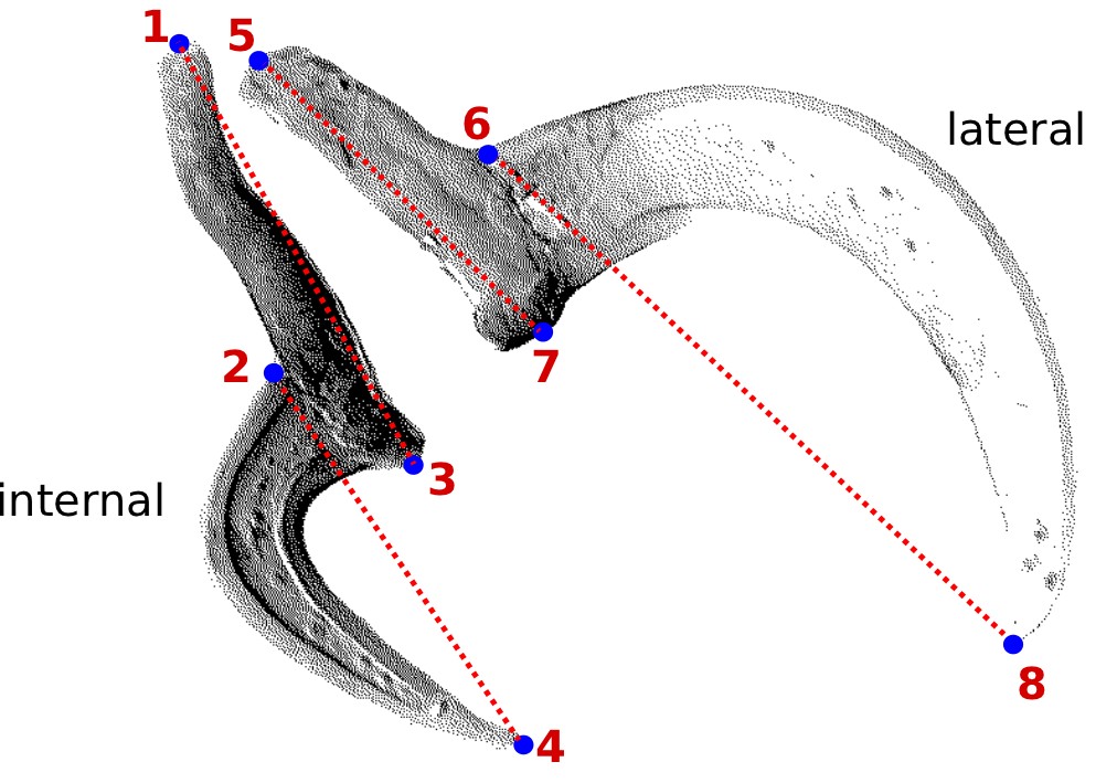
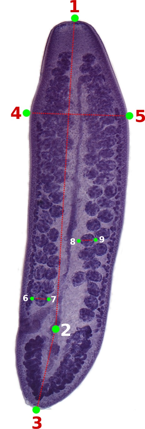
You should start by defining the landmarks that would allow you to calculate the distances (measurements) you need (Figure 2). In the example below, we want to obtain the measurements from handles and prongs of the internal and lateral bothridial hooks. Accordingly, we defined 8 landmarks (Figure 2). WormBox allows you to set as many as landmarks as you need (or wish), but you should always be careful and minimize the amount of landmarks for practical reasons.
Getting started with WormBox
Once you have a good idea of the measurements you want to take and the landmarks required to do that, you should compile within a folder all the images you want to extract the measurements. We provide a folder called “hooks” that we will use in the first part of this tutorial. The images in this folder have the hooks from which to obtain the measurements defined in Figure 2. Ultimately, the images should be all scaled, preferentially using ImageJ or Fiji/ImageJ. WormBox will inform you whether it recognized the scales in your images. If WormBox does not recognize the scale, it will ask you to set up the scale. Here are the steps you should take to fully complete the first part of this tutorial (PDF):
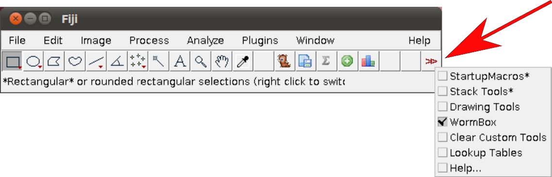
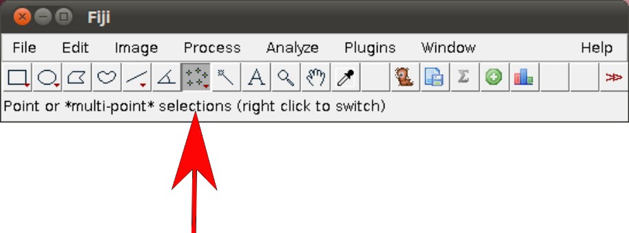
- Step 1. Start Fiji/ImageJ and enable WormBox in the switch to alternate macro tool sets (Figure 3).
Once the plugin is enabled, 5 new icons will become available to you with the following function:
![]() Initialize landmark setup and/or load ROI (Region of Interest) to images.
Initialize landmark setup and/or load ROI (Region of Interest) to images.
![]() Save landmark positions.
Save landmark positions.
![]() Count meristic variable.
Count meristic variable.
![]() Add new landmarks.
Add new landmarks.
![]() Run WomBox Analyzer, to compile measurements to *.cvs file.
Run WomBox Analyzer, to compile measurements to *.cvs file.
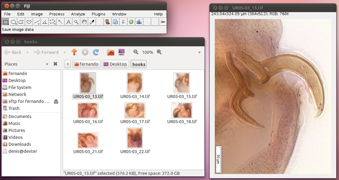
- Step 2. Open the first image of your working folder. You can do that by either dragging the image into the Fiji/ImageJ main menu area (gray area) or by using File/Open.
NOTE: Files should be in *.tif format and the extension should be in lower case. WormBox will recognize all major images formats recognized by Fiji/ImageJ. However, if the original image is not in *.tif format, or if the extension is written in upper case, WormBox will make a copy of the image and save it as *.tif after processing.
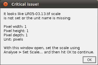
- Step 3. Scaling images. If your images are not scaled by Fiji/ImageJ or, although scaled using a different software, Fiji/ImageJ did not recognize the scale, WormBox will require that a scale is provided and the warning window below will be presented.
To scale the image in Fiji/ImageJ you will have to follow these steps:
- Step 3a Select the “straight” tool to draw lines. =
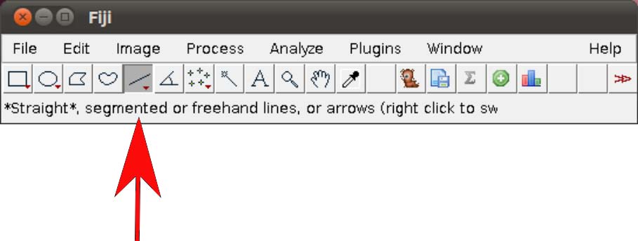
- Step 3b Draw a straight line using as reference the scale bar embedded into the image.
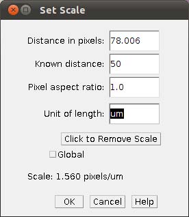
- Step 3c In the main menu, select Analyze/Set Scale and provide the known distance (i.e., 50)
and the unity of the length (i.e., um).
NOTE: It might be easier to have all images scaled before setting up landmarks. But that is not mandatory, you can provide the scales as you work in each image.
- Step 4 Placing landmarks. If you have opened a image and WormBox has recognized the scale, you are ready to define and/or place the landmarks you desire to obtain the measurements you want. Press the button to load ROI from the WormBox tool set. If this is the first time you are using WormBox for the images within a given folder you will have to define the number of landmarks you will be working.
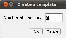
As we mentioned above (Figure 2), we will need 8 landmarks for the measurements we are planning to take from the hooks. By selecting 8 and pressing “OK”, we will define a template with eight landmarks which will be used for all images in this folder (Figure 9A). A file called RoiSet.zip will be created and all landmarks will appear on the left part of the image.
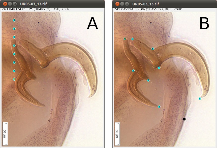
Once the landmarks have been defined or loaded, all you have to do is to drag the landmarks to its right position using the mouse (double-click on the landmark you want to move and drag; if you prefer, you also can select the landmark`s number on the box (ROI) and after that click once on the landmark in the figure and drag it) (Figures 2 and 9B) and then save it using the icon in the macro tool set menu of WormBox. After saving the image, WormBox will wipe the landmarks from the image. However, all information will be still there, saved in associated files with extensions *.txt and *.zip. These files will be used to compile the information after you process all images and SHOULD NOT BE REMOVED – unless you want to wipe out all the data. If you desire to verify and or modify the positions of the landmarks, just reload the ROI using the icon in the macro tool set menu of WormBox.

NOTE: WormBox allows you to delete any landmark if you feel that a given measurement should not be taken from a given image. All you have to do is to place the landmarks that you consider that should be included in the image and use the ROI manager to delete the ones that should not be taken into account. In its final stage, when WormBox will parse the images to compile the measurements, images for which one or more landmarks are missing, will still be used. WormBox will attribute “NA” for cells in which the distance could not be calculated by the lack of landmarks in the *.cvs file (see below).
NOTE: WormBox allows you to add landmarks if you want to. All you have to do is to click on the icon in the macro tool set menu of WormBox, write the number of landmarks you want and press ok. The new landmarks will appear on the image. You only can add landmarks in the end of your landmarks that already exists, for example, if you have landmarks 1,2 and 3 and you add more 2 landmarks, this landmarks will be the number 4 and 5. If you count some structures, this will be interpreted by WormBox like a landmark, for example, in this case we have 5 landmarks and 2 counted structures. This two structures counted will be landmarks 6 and 7, so, if you add 2 new landmarks, this will be the number 8 and 9, and not the 6 and 7. The ideal situation is add all landmarks you want before count structures.
- Step 5 Compiling the data from images. Once you have processed all images (in this particular example it should take less than 10 minutes to process all 8 images) you will have to write a configuration file to run the compiling tool of WormBox. The configuration file should be in a plain text format. Thus, do not use Word or any other text editor the leave hidden characters into the text. Linux users could use nano, vim, or Geditand, among others. Mac users could use TextEdit, Wrangler, or nano, among others. Here is an example of the file:
internal_handle:1,3
internal_prong:2,4
lateral_handle:5,7
lateral_prong:6,8
Each line should contain the name of the variable, followed by “:” and at least two landmarks separated by comma defining the two points from which WormBox will calculate the distance.
NOTE: You can use more than two land marks for a single variable. For instance, your configuration file could have a line like this: “variable_x:1,2,3,4”. In this case, the measurement for “variable_x” will be the sum of the distances between 1–2, 2–3, and 3–4.
Once you have written your configuration file (e.g., hooks_measurements.conf) and saved it, run the WormBox Analyzer (see definition of icons above). First, WormBox will ask you the target folder in which your images have been processed (Figure 10A); and then the name of your configuration file (Figure 10B).
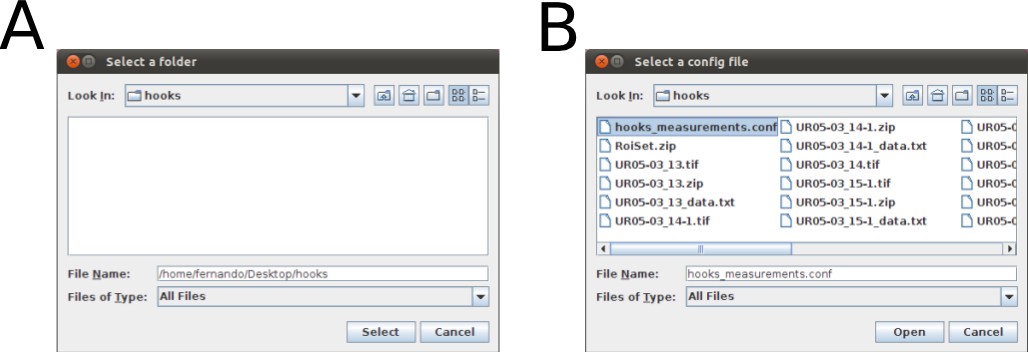
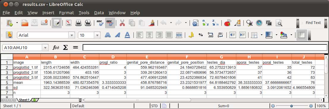
Finally, you will have to specify the output file name. WormBox will generate a *.csv (comma separated values) text file that can be opened in any spreadsheet software (e.g., Excel, OpenOffice, among others) as demonstrated in Figure 11.

The summary results will contain a column with the image names and each variable will be displayed in a separated column. The three last lines of the file will compile the average, standard deviation and sample size of each variable. Cells with “NA” (as Non Available) denote measurements that were not taken due to the lack of associated landmark(s).
More on WormBox (advanced features)
Now we will explore some other features of WormBox. We provide a folder called “proglottids” upon which we base this second part of the tutorial. Within this folder you should find 3 images of loose proglottids of Potamotrygonocestus, all of which have been scaled using Fiji/Image.
In Figure 12 we depict the landmarks we wish to use to compile length and width of the proglottids, position of the genital pore, and testes diameters. We also will compute the number of testes for each proglottid. Thus, we will make use of the counting tool in WormBox, which we have neglected in the first part of the tutorial. Except for the fact that we are using two sets of landmarks to compute testes diameter, and that the total length of the proglottids will be calculated the sum of two distances (i.e., 1–2 and 2–3), you should have no problem with that if you went through the first part of the tutorial. It is true that the configuration file will have to specify that; which will be addressed latter. Thus, let's see how we count structures using WormBox.
Counting structures:
Before starting the use of the counting toll of WormBox, you should:
- Define the number of landmarks you need.
- Place them in the right positions.
- Save image (required).
The steps above have been described in the first part of the tutorial. If you have any difficulties, please go back and have a quick look above. To start counting, you have to enable the function to count meristic variables (icon with Σ sign). By doing that, you will turn on the multi-point tool of Fiji/ImageJ and a window named “action required” will appear.
Once the counting tool is on, all you have to do is to position your mouse on top of the structures you want to count and click the mouse. Here, we will count two sets of testes: poral and aporal ones. As you start clicking on top of the testes, let's say on the aporal side, landmarks in yellow will provide the counting (Figure 14).

After concluding counting the aporal testes, you should click on “OK” on the window for “Action Required” and this will prompt WormBox to ask you to name of the variable you just counted (e.g., aporal_testes).
NOTE: Watch out for spelling error here otherwise the script will consider them as different variables. It is important to inform you that the script is case sensitive. Thus, “testes” and “Testes” will be understood as two different variables.
Now, let us count the other set of testes, i.e., poral testes. You can start by loading all you have done thus far by pressing the icon to load ROI into image. If you load the ROI, you should have something like Figure 15.

The image should display all landmarks for calculating distances and counting, and the ROI manager should have a list of all landmarks and variables. Now proceed to count the poral testes by enabling the counting tool and repeating the steps you did before in which you count the aporal testes. You should repeat all the steps above for the other remaining (2) images.
Compiling results (complex version)
As explained above, you will need to specify a configuration file to parse all the information you implemented in each image. Here we will apply a configuration file a bit more sophisticated than before. Within the configuration file, we will not only obtain euclidean distances between landmarks but also specify new variables based on operations of those distances.
Below we provide a example of configuration file to illustrate this capability of WormBox. For explanation proposes, each line is specified by a number (e.g., #1), which should not be in the configuration file:
#1  length:1,2,3
#2  width:4,5
#3  progl_ratio:${length}//${width}
#4  genital_pore_distance:2,3
#5  genital_pore_position:${genital_pore_distance}*100/${length}
#6  testes_dia:6,7
#7  testes_dia:8,9
#8  aporal_testes:count
#9  poral_testes:count
#10 total_testes:${aporal_testes}+${poral_testes}
Here is what this configuration file will do with the data you compiled for each image:
- Lines 1 and 2 (i.e., #1 and #2) will calculate the length and width of your proglottid, which except for the fact that the length is being calculated by the sum of two distances (i.e., 1–2 + 2–3), they are the kind of distances you calculated before in the first part of this tutorial.
- Line 3 provides something new. Here we defined a new morphometric variable,”progl_ratio“, which is equal to the floored quotient of length and width of the proglottid; that is, its ratio. To operate with variables there are few rules you must follow:
- You can only operate with variables that were defined before. That is, line 3 could not be written prior to lines #1 and #2.
- The syntax for operating variables should be “${name_of_variable}”.
- The operator used in WormBox are basically those available in Python:
| Operation | Result |
|---|---|
| x + y | sum of x and y |
| x - y | difference of x and y |
| x * y | product of x and y |
| x / y | quotient of x and y |
| x // y | floored quotient of x and y |
| pow(x, y) | x to the power y |
| x ** y | x to the power y |
- Other lines that make use of this property are lines 5 and 10 in which we calculate the genital pore position and the total number of testes, respectively.
- Next, we should comment lines 8 and 9. These two redundant lines specify the distances for testes diameter (i.e., 6–7 and 8–9). For those, when WormBox parse the information of an image, it compiles the mean value between 2 or more pseudo-replicates (or repetitive measures).
Finally, meristic variable are defined by its name followed by “:count”. Examples of that are the testes counts defined in “aporal_testes” and “poral_testes”, lines 8 and 9, respectively.
The final results should be something like this:
Cestode Taxonomy and Statistics
As show above, like other tools available out there, WormBox compute summary statistics from your images. This summary includes measures of central tendencies and dispersion of your data, as well as averages of pseudoreplicated data. All these concepects will be discussed below. If you gathered morphometric data and summarized the information using statistics you have to think what those values mean to you – truelly what can you do with them. Are they simply a description of your data? or Are they sample statistics from which you are trying to estimate parameters of population? These are two fundamentally different approaches in statistics pertaining to descriptive and inferential statitistics – respectively. This dichotomy may, at first glance, be trivial and uninteresting, but for statistical theory they are not! If you put these questions into the context of taxonomic descriptions, and you state:
You should then consider whether these statistical statements only describe your data (i.e., the morphometric attributes of a type series, for instance) or they were calculated with the intent of estimate values of all individuals that belong to the taxon you just described – therefore, potentially diagnostic characters. If you consider them to be descriptive statistics, these numbers only describe the distribution of what is shown before us and, as such, cannot be used to draw any specific conclusions based on any hypothesis or test (Klazema, 2014). On the other hand, if they were meant to be used as an inferential statistics tool, these numbers must come from one or more representative samples from the set you are interested and subsequently be used to test statistical hypotheses.
This rational has serious implications on the use of morphometric data as diagnostic characters. If the statistics you reported were summarized under the premise they were only descriptive, it would be inconsistent to use them as diagnostic characters. To be used as diagnostic characters, it is implicit that your samples allow valid estimation of population parameters that represent your taxon concept.
The present day taxonomic literature on cestodes (as in many other groups) are flooded with summary statistics. If you look historically, you will find a clear trend in which throughout the years new variables – structures measured and/or counted – have been added into descriptions; as if a well performed taxonomic description depended on larger numbers of assessed variables! On the other hand, little effort has been put into increasing sample sizes and/or in their statistical validity. Whether taxonomists working on these groups have ever reflected up on the distinction between descriptive and inferential nature of the data they present and how that would affect their practice is an open question. The available literature suggests that, as a community, we seem to loosely jump from one context to the other as we please without statistical rigor. In the sections below, we will illustrate the major problems we recognize on the use of statistics in taxonomy of cestodes and propose some guidelines which we consider more appropriate for the data we compile.
The tradition and implications
It would be fair to start with an example in which one of us is involved so that we are not criticized for hiding our own mistakes while pointing the others. We should recognize that all of us are bound follow tradition without critical evaluation at some point. Few years ago, Marques et al. (2012) described a new taxon called Ahamulina catarina – a new genus and species of diphyllidean found in deep water catsharks off the coast of Brazil. Here is what they stated in part of the description of this new taxon based on on 9 complete and 6 incomplete whole-mounted specimens, cross-sections of 2 proglottids (Marques et al., 2012:55):
If you are not familiar with this notation, it follows the format: maximum – minimum values, followed by mean ± standard deviation and sample size, between brackets. These numbers intent to provide statistics for measurements of structures. The mean is a statistic of location, in this case associated with the central tendency of the distribution. The standard deviation is a statistic of dispersion, which provides information about the spreading of values around the mean (see Sokal and Rolf, 1996; among other textbook on Statistics). Below we provide few other examples from different groups of cestodes to show that the notation used by Marques et al. (2012) is standard practice in the field:
Cirrus sac widely pyriform, 140–200 long and 90–170 wide, its length representing only 14–21% of proglottis width (x = 17%, n = 26) ...
Ovary width represents 72–79% (x = 76%, n = 25, CV = 3%) of proglottis width ...";
"..., prebulbar organs present, small; bulbs elongate (Fig. 3), bent,
thick-walled, 600-760 (649 ± 53; n = 22) long by 100-130 (117 ± 10; n = 22) wide, ...";
There are two components we are concerned and will discuss in detail below. One is related to the concept of pseudoreplication (sensu Hurlbert, 1984) – which seems to permeate this literature. The other concerns the implicit assumptiom of that the data have a normal or at least bell-shaped distribution. We will start with the problem of pseudoreplication, then we will revisit some of the properties of the parameters that describe statistical distributions, and finally, we will try to convince you that there are more informative metrics that we could adopt when describing our morphometric data.
Pseudoreplication
One of the fundamental assumptions of most statistical techniques is that observations are independent of one another (Hurlbert 1984). Pseudoreplication typically occurs when the number of observations are treated inappropriately as independent replicates. Observations may not be independent if ( i ) repeated measurements are taken on the same subject, ( ii ) the data have a hierarchical structure, ( iii ) observations are correlated in time, or ( v ) observations are correlated in space (Millar and Anderson,2004; but see Schank and Koehnle, 2009). Pseudoreplication is not uncommon in other areas of research (Hurlbert 1984, Millar and Anderson,2004; Lazic, 2010; among others) and a lot of debate has been published in the literature since Hurlbert (1984) called the attention of ecologists to the problem. Since then, researchers either acknowledged the problem and tried to avoid it by redefining experimental or sampling design and/or relying on more complex statistical models or, sadly, simply noting its existence and then keep doing what was done before (see Schank and Koehnle, 2009; Zuur et al., 2010). We hope you do not choose the latter.
We should go back to the taxonomic examples above and compare the number of individuals (whole worms) available for each description and the sample size reported for each variable. It should be obvious that for some variables (i.e., structures or part of thereof), the descriptive statistics is based on a larger number of observations than the amount of individual worms available to the investigator. For instance, Marques et al. (2012) reported that the mature proglottid of Ahamulina catarina was 728–1,892 (1,153±228; 47) long by 291–586 (460±70; 47) wide, all based on 47 observations. How could that be if they had only ”9 complete and 6 incomplete whole-mounted specimens“? A hint: they took more than a single measurement from a single specimen. This is pseudoreplication.
It is true that most statistical techniques assume that observations are independent – but but we do not use at all those that account for dependency. One could suggest that maybe the examples above are not such a terrible sin after all. However, all statistical metrics we are using assume independence and, for inferencial purposes would also require special attention to sample sizes and random sampling. Thus, repeated measurements taken on the same subject violate one of the major assumption and statistic. We will provide you an example to illustrate how pervarsive can be the introduction pseudoreplication to the description of your data – just in case the violation did not convince you already that you should avoid it. Consider the data presented in Table 1.

The table above starts 15 random numbers withdrawn from a log-normal distribution (meanlog = 3, sdlog = 0.35). The theoretical mean and median of the lognormal can be easily be calculated 1) and in this case are mean = 21.35423 and median = 20.08554. We will refer to these values as population parameters. Differences between mean and median indicate that the data deviate from symmetric distribution (e.g., normal, we will come back to that soon). When we calculated the mean and median from our sample (15 datapoints), we obtained the values of 20.56 and 20.30; respectively, which will refer as sample estimated parameters. Due to the finite sample size, we observe that the population parameters are not identical to those estimated from the sample. Additionally, the differences between central tendencies estimated from the sample are not as discrepant from each other when compared to those obtained for the population. Hence, based on the sample, the data seem not to deviate as much from a symmetric distribution as the population parameters would suggest.
In Table 1, the columns Examples 1–4 include incremental amounts of pseudoreplication for 6 randomly chosen individuals (highlighted in yellow). For each example, pseudoreplication was introduced so that the mean value of the original individual was maintained. For instance, for “individual_1” the original value was 12.99, and the mean for all introduced pseudoreplication (i.e., (12.99+11.48+13.50+14.00)/4 = 12.99) has the same value.
This example show some undesirable (not to say, statistically unsound practice) effects of pseudoreplication. It is noticeable that all parameter estimation for central tendencies and spread of the distribution (i.e., stardard deviation) dissociate from the original values of the sample and the population. Note that in Example 4, the mean and the median are identical, indicating that the data follow a symmetric distribution when in fact it was generated under a log-normal model. Finally, as the parameter that measure dispersion (or spread) of the data, standard deviation – although inappropriate for asymmetric distributions will be demonstrated latter –, tends to get smaller (i.e., reducing the spread, which is a measure of variability in the data) because repeated measurements from the same specimem will introduce less variability than adding measurements from additional specimens.
Thus, as a rule, pseudoreplication will ( i. ) introduce bias, ( ii. ) reduce accuracy, and ( iii. ) violate the basic premises of statistics. All of which, we should avoid at all costs.
The take home message of this section is simple: if you desire to increment your sample size, do that by sampling data for more individuals – unless you are interested on intra-individual variation, but that is a different ball game and beyond the scope of this section. If you have pseudoreplicates in your dataset, the simplest way to correctly deal with them is to average them by individuals – along the same line that the application WormBox (above) deal with them.
Distributions and summary statistics
Descriptive statistics help to describe and summarize data in a meaningful way such that, for example, patterns might emerge from the data. For instance, when Marques et al. (2012:55) stated that Ahamulina catarina is an apolytic worm 23–45 (30±7; 8) mm long, the notation presented the authors' summary the data compiled from 8 mature worms, from which they obtained the following data: 3.233, 25.237, 33.651, 27.342, 25.117, 44.779, 27.473, and 33.323 mm.
The notation “23–45 (30±7; 8)”, so common in our field (see examples above), is the results of univariate analyses that entail some assumptions about the property and nature of the data. By definition, univariate analysis involves the examination across cases of one variable at a time. The goal of this analysis is to provide some information on the distribution, central tendency and the spread (variability or dispersion) of the data, for those are the three major characteristics of a single variable.
Distribution
The distribution is a summary of the frequency of individual values or ranges of values for a variable. One of the most common ways to describe a single variable is with a frequency distribution (Trochim, 2006). In Figure 1A you will find the frequency distribution of the total length of Ahamulina catarina compiled by Marques et al. (2012). Another way of describing the distribution of this data would be by a histogram of the probability densities (Figure 1B). This is simply a rescaling of the y-axis to make the areas of the bars sum 2). Under the density scale, the probability of sampling at random an observation that has between 30 and 35 mm is equal to the proportion of the summed area of the bars that encompasses this interval in the histogram. Finally, in Figure 1C we represent a theoretical Probability Density Function (PDF), assuming a normal distribution (i.e., the most popular bell-shaped, symmetric distribution) defined by two parameters estimated from the data, one which matches the theoretical central tendency and the other that matches the theoretical spread – which we will discuss in detail below. For density functions, the area below the curve defines the probability of withdrawing a random sample witing that area. Hence the total area under the curve is one, which is the same to say that a measure has a probability of 1.0 to assume one of the possible values in the range defined by the distribution.

Figure 1. Distribution of 8 measurements of total length for Ahamulina catarina used in its original description. A. Frequency distribution of the data. B. Probability distribution of the data. C. Mathematical distribution or Probability density Function of a normal distribution model assuming estimated parameters from the data.
Central Tendency
The central tendency of a distribution is an estimate of the “center” of a distribution, and as such should give you an idea on what particular value or interval of values most of your samples reside. This is an useful metric, especially when you have no access to a graphic representation of the distribution. In fact, parameters such as central tendency, dispersion and skewness should try to do the best description of your distribution. According to Lane at al. (2014), there are three main ways of defining the center of a distribution, and the parameters used to inform us of the central tendency of a distribution rely on those different definitions. One possible way would be to consider de central tendency is the point at which the distribution is in balance. An alternative measure would be considering the center of a distribution the value that minimize that absolute deviations (differences). Finally, the concept of central tendency could be based on the value that minimizes the sum of squared deviations.
There are three major types of measures of central tendency: Mean (arithmetic), Median and Mode. The arithmetic mean is the most common measure of central tendency in our field. The theoretical mean is the sum of each in the range of the distribution times the probability the distribution assigns to it 3), and is related to minimizing the sum of squares of deviations from the central tendency. The median is also a frequently used measure of central tendency – although in our field rarely so. The median, also referred as the 50th percentile as it halves the area of the distribution, is the midpoint of a distribution and is based on the concept of the sum of the absolute deviations. Finally, the mode is the most frequently occurring value.

Figure 2. Central tendency for Ahamulina catarina based on the distribution of original data. A. Position of the mean on the normal density function. B. Position of the median on the normal density function. C. Position of the mean and median on the empirical frequency distribution.
Under a normal distribution model (see Figures 2A-B) mean and median are equal. However, as the distribution deviates from normality and becomes asymmetric (skewed, as data suggest in Figure 2C) the mean differs from the median. For instance, if the mean is larger than the median, that is a sign that your distribution has a positive skew – the tail on the right side of the distribution is longer or fatter than the left side one.
Dispersion
Dispersion refers to the spread of the values around the central tendency and indicates how spread out the data is. As for the central tendency, there are several measures of dispersal. In fact, we commonly use two of them as can be seen in the taxonomic examples we provided above. Recall that the notation “23–45 (30±7; 8)”, express the range (i.e., 23–45), the mean (i.e. 30), the standard deviation (i.e., 7), and the sample size (i.e., 8) for a given variable. Of those, range and standard deviation are two measures of dispersion. Below we explain some of their properties and present other measures of variability.

Figure 3. Estimated probability density function for normal distribution for total length of Ahamulina catarina based on parameters estimated from empirical data by Marques et al. (2012) showing different measures of dispersion. Boxplot is in green. Dark red area under the curve represent the area of 1 x standard deviation and lighter red area 2 x standard deviation. Red solid vertical line represents the mean. Vertical dashed blue lines indicate lower ad upper limits of the range from 1000 random numbers drawn from the distribution. The theoretical range of the normal can not be depicted because it is minus inifinity to infinity.
The range is one of the simplest measures of dispersion. In the sample it is obtained by subtracting the minimum score from the maximum score of your data. For instance, in Figure 3, the small circles in the plot represent values distributed at the beginning and at end of a sample of 1000 values. The vertical dashed blue lines in that plot indicate lower ad upper limits of the observed range. A practical shortcoming of the observed range is that it is very sensitive to extreme values or outliers (possible spurious observation, see below). Thus if you have an extreme value in your sample associated with error, it will spread spuriously the range of your variable. A more subtle shortcoming is that the observed ranges are very poor estimates of the true range for most distributions, because it is hard to estimate the true maximum and minimum values of a given measure. Usually, as we increase our sample there is always a probability to find a value that is larger than the largest already found (or smaller than the current minimum). As tiny as this probability can be, if is there any chance to get a lower/larger value the observed range has very few information on the true range. One of the reasons that most of the theoretical distributions span from/to infinity is to recall us of that.
Dispersion can also be defined on the basis of how close the scores in the distribution are to its central tendency, specially the average squared difference score from the mean – a measure of variance:
<latex>
\begin{center}
\begin{equation*}
& & & & s^2 = \frac{\Sigma (x_i-\bar x)^2}{N}
\end{equation*}
\end{center}
</latex>
where <latex>\bar x <\latex> is the sample mean, N is the sample size, and <latex> x_i<\latex> each observed value. Usually the sample variance is calculated as the sum of squared differences divided by N-1:
<latex>
\begin{center}
\begin{equation*}
& & s^2 = \frac{\Sigma (x_i- \bar x)^2}{N-1}
\end{equation}
\end{equation*}
</latex>
The reason for the subtraction of 1 to the sample size is that the variance is a biased estimator of the true variance for small sample sizes and N-1 provides the correction necessary to approximate the estimator. The bias vanishes as the sample increases. It is more common to report the bias corrected form, which is the correct choice if you want to make statistical inferences about the population (see below).
The units of the variance are the square of the original measure. For instance, the variance of lengths are areas. To avoid such oddity, the most common measure of dispersion is the square root of the sample variance; the sample standard deviation:
<latex>
\begin{center}
\begin{equation*}
& & & & \sigma = \sqrt{\s^2} = \sqrt{\frac{\Sigma (x_i-\bar x)^2}{N}}
\end{equation*}
\end{center}
</latex>
, where as the bias-corrected estimate is
<latex>
\begin{center}
\begin{equation*}
& & \textit{s} = \sqrt{s^2} = \sqrt{\frac{\Sigma (x_i-\bar x)^2}{N-1}}
\end{equation}
\end{equation*}
</latex>
The sample standard deviation is specially informative when the distribution is normal because 68% of the normal distribution is within one standard deviation from the mean and 95% within 2 standard deviation (Figure 5). Hence, using the sample mean and the sample standard deviation estimates of these paraneters of undelying normal, we can guess that about 68% of the individuals in the population are in the range mean ± sd.

Figure 5. The area under the normal distribution can be defined in units of standard deviation. The central 68% of the distribution is within the mean ± one standard deviation, while 95% of the area is within mean ± one standard deviation. Hence, if we assume a normal distribution we can use the sample mean and standard deviations as estimates of the parameters of the distribution and guess the proportion of individuals expected in a given interval.
All these measures of dispersion give distinct information about the data you are describing and some interpretations requires that some assumptions are met. As will be discussed in more details below, box plots do not make assumptions on the underlying distribution – therefore, it is non-parametric –, whereas standard deviation is more informative under a normal distribution model (or other symetric distributions). As can be seen in Figure 5, the interquartile range is more restrictive than one standard deviation, since the first accounts for 50% of the distribution while the latter 68.2%. If your data is normally distributed, all of those measures will provide a reasonable account of dispersion and adequate description, and the only consideration you have to make is which measure you think is more appropriate to be used for what you desire to describe. However, if your data deviates form a normal distribution, then imposing the model to your data will render an unrealistic description of it and hide information that could be important.

Figure 6. Distribution of total length of Ahamulina catarina depicted by a empirical frequency distribution histogram (in gray), probability density function under normal distribution model with shaded area representing one standard deviation, and the box plot (green).
Back to our example, Marques et al. (2012:55) reported in their original description of Ahamulina catarina that those worms had 23–45 (30±7; 8) mm in length. Applying the concepts we just discussed above, we can infer based on their report that within that sample of 8 worms, the smallest one was 23 mm long, the largest one 45, the average size was 30 mm, and ~68% of that sample had 30±7 mm of length (i.e., between 23 and 37 mm). For these data, the estimates of central tendencies, mean and median, indicate that the distribution has a positive skew. Therefore, suggesting that the normal distribution model is not the best description of the data. Note that the box plot provides a more accurate description of them and could be textually provided by the five-number summary (Tukey, 1977) 23.2, 25.2, 27.4, 33.5, and 44.7, for minimum, 1st quartile, median, 2nd quartile, and maximum. The advantage of this notation is that it does not require assuming that your data is normally distributed and will be more informative when your data is not normally distributed.
Is normal distribution a required assumption for reporting morphometric data?

Figure 7. The probability distribution of discrete random variables for three Neotropical freshwater species of Rhinebothrium (raw data from Reyda & Marques, 2011).
Whether you are dealing with discrete or continuous variables defines also the probability distribution you should consider to describe your data. Accordingly, different models of probability distributions exist and are generally classified as discrete probability distributions or as continuous probability distributions. As a rule, if a variable can take on any value between two specified values, it is called a continuous variable as lengths, areas and volumes. Otherwise if a variable is a count it is called a discrete variable. Normal distribution is a continuous distribution. Thus, a priori it should not be assumed for discrete variables – although it is true that in some cases the distribution of some discrete variables may approximate a normal distribution. Be that as it may, in many cases it will not, and one should consider why should we assume a distribution that, from the start, was not intended to provide proper description of our data. Consider the plots in Figure 7.
The distribution of proglottids for Rhinebothrium paratrygonyi, for instance (Figure 7), is better explained by a negative binomial discrete distribution (AIC4) = 672.5385) than two other continuous distributions, normal and log-nomal (AICs = 673.589 and 674.4242, respectively). If you consider the distributions of the number of testes for R. brooksi and R. brooksi it is clear that they cannot be described by a normal distribution.
The justifications for the assumption that morphological continuous characters have normal distribution can be traced to Fisher (1918). He argued that the additive effect of many random environmental variables interact with genotypes producing a range of phenotypes at the same time that phenotypic variation could be associated genetic additive variation at many loci. Under those set of assumptions of random interactions, we should expect a normal distribution for many phenotypic traits (see also Templenton, 2006). Although this may be so, in many instances the approximation to a normal distribution will depend on large sample sizes which is difficult to obtain in our field. For some discrete characters, even large sample sizes will not converge the empirical distribution to a normal model – as is the case for the testes numbers for those 2 species of Rhinebothrium in Figure 7.
Back to the question of this section, we think that normal distribution is not only unnecessary to describe your data but also that in some cases it is not appropriate. In the next section, we provide a tool to compile the five-number summary, which we think that would do a better job as a descriptive statistic parameters for taxonomy.
Five-number summary
The five-number summary was proposed originally Tukey (1977) as a set of measures for descriptive statistics. The five numbers include the median, the limited is the interquartile ranges and the minimum and maximum values excluding those that are considered outliers, which by his definition are those that exceed the lower and upper limits of the inner fence. The later is arbitrarily defined as 1.5 x IQR (see Figure 4). Although since its conception, the so called “five-number summary” has suffered some modifications and or the inclusion of other metrics (such as mean, for instance), we think that those numbers might do a better job than the standard traditional use of max–min (Mean ± standard deviation). This is particularly true for skewed distribution and also for discrete variables. Finally, the five-number summary, often graphically represented by box plots, make no assumption about the distribution.
With that in mind, we devised the script written in R, which we think that might be a useful tool for you to explore your data. Below we explain how the script works.
Consider that you have compiled the following data:
specimen	n_testes
specimen_1	2
specimen_2	3
specimen_3	3
specimen_4	5
specimen_5	5
specimen_6	6
specimen_7	6
specimen_8	7
specimen_9	9
specimen_10	10
specimen_11	12
specimen_12	12
specimen_13	13
specimen_14	13
specimen_15	14
If you are familiar with R, you could just execute:
>n_testes  <- c(2,3,3,5,5,6,6,7,9,10,12,12,13,13,14)
> summary(n_testes)
and you would obtain:
Min. 1st Qu.  Median    Mean 3rd Qu.    Max.
2       5       7       8      12      14
This summary shows that the minimum valuer for your variable is 2, the maximum is 14, that the distribution is centered in the median 8 and that 50% of your samples have from 5 to 12.
If you are interested in looking at how the box plot for this variable looks like, run:
>boxplot(n_testes)
and R would return you the following plot:

This is the graphical representation of the five-number summary above.
The script available here does somewhat the same, but allows you to explore your data in a more effective way. To work with this script, there are few things you need to know. Here they are:
Structure of the input file
The input file must be a text format file, TAB delimited, and have at least three columns: specimen, group and variables. It should look like this:
specimen	group	n_testes	total_length
specimen_1	host	2		2.1
specimen_2	host	3		2.2
specimen_3	host	3		2.2
specimen_4	host	5		2.3
specimen_5	host	5		2.4
specimen_6	host	6		2.5
specimen_7	host	6		2.6
specimen_8	host	7		1.2
specimen_9	host	9		5.5
specimen_10	host	10		6.7
specimen_11	host	12		6.7
specimen_12	host	12		7.8
specimen_13	host	13		8.0
specimen_14	host	13		8.0
specimen_15	host	14		9.0
You can have as many variables you want as well as many groups. Groups are identification tokens for specimens, let us say, host species or localities. One important thing to remember, the script averages out pseudoreplication. Thus, if the first column has more than a single specimen under the same name within a given group, the script will compute the mean value for the specimen and consider a single data entry – for the reasons discussed above.
Modes of execution
In its simplest form, the script should be executed in a shell terminal with the following sintax:
Rscript compile5numbers.r input_file
For example, the data above was in a file called example.txt, the execution would be:
Rscript compile5numbers.r example
This would return the file called my_out.csv, which is a file in a CSV (comma separated value) format – therefore you can open it in a spreadsheet application of your choice, with the following content:
| stats | n_testes | total_length | |
|---|---|---|---|
| 1 | LowerValue | 2 | 1.2 |
| 2 | 1stQ | 5 | 2.25 |
| 3 | Median | 7 | 2.6 |
| 4 | 3rdQ | 12 | 7.25 |
| 5 | UpperValue | 14 | 9 |
| 6 | N | 15 | 15 |
The problem with this syntax is that you run the risk of overwriting output files, Thus the safest execution syntax would be
Rscript compile5numbers.r example -prefix any_word
The argument argument “any_word” for the option ”-prefix“ attaches the term at the beginning of each output file. For example, is you execute
Rscript compile5numbers.r example -prefix fernando
The same output file as before would be called fernando_out.csv.
This script can include as output files boxplots. To do that you have to include the option -boxplot into the command line, like:
Rscript compile5numbers.r example.txt -boxplot -prefix fernando
For the data above, this command line would generate a CSV file (Scalable Vector Graphics) called fernando_boxplot001.svg with the following box plots:

The last feature of this script is its ability to compute statistics and draw plots comparing groups and variables. To illustrate that, let us modify the input file attributing the specimens to two different hosts. Something like:
specimen	group	n_testes	total_length
specimen_1	host_1	2	2.1
specimen_2	host_1	3	2.2
specimen_3	host_1	3	2.2
specimen_4	host_1	5	2.3
specimen_5	host_1	5	2.4
specimen_6	host_1	6	2.5
specimen_7	host_1	6	2.6
specimen_8	host_2	7	1.2
specimen_9	host_2	9	5.5
specimen_10	host_2	10	6.7
specimen_11	host_2	12	6.7
specimen_12	host_2	12	7.8
specimen_13	host_2	13	8.0
specimen_14	host_2	13	8.0
specimen_15	host_2	14	9.0
The option that allows you to compare groups per variable is called -groups, obviously! If not evoked, the script will treat the data as a single class group and the results would be the same as before even if your dataset has class groups defined. Here is the an example of command line evoking the comparative analysis:
Rscript compile5numbers.r example_hosts_groups.txt -boxplot -groups -prefix fernando_2
This analysis generates 3 files: fernando_2_out.csv, fernando_2_boxplot001.svg, and fernando_2_boxplot002.svg. The first one contains the summary statistics for each groups, and the other two files are SVG figures containing box plots for each variable.
Here is the structure of the summary statistics:
| group | stats | n_testes | total_length | |
|---|---|---|---|---|
| 1 | host_1 | LowerValue | 2 | 2.1 |
| 2 | host_1 | 1stQ | 3 | 2.2 |
| 3 | host_1 | Median | 5 | 2.3 |
| 4 | host_1 | 3rdQ | 5.5 | 2.45 |
| 5 | host_1 | UpperValue | 6 | 2.6 |
| 6 | host_1 | N | 7 | 7 |
| 7 | host_2 | LowerValue | 7 | 5.5 |
| 8 | host_2 | 1stQ | 9.5 | 6.1 |
| 9 | host_2 | Median | 12 | 7.25 |
| 10 | host_2 | 3rdQ | 13 | 8 |
| 11 | host_2 | UpperValue | 14 | 9 |
| 12 | host_2 | N | 8 | 8 |
Here are the plots generated5):

The results of this analysis is two plots as shown above. On you left you have the comparative distribution of the number of testes of these two groups of worms. Note that the ranges do not overlap. What does that mean? Well, we would say that the ranges of testes numbers of those specimens do not overlap. That is it. On your right, you have the distribution of the total length of those two groups. There is something worth a comment on that graph. Observe that the box plot recognized an outlier for the specimens attributed to Host 2. This is a useful tool of this script – of the box plot to be fair – that would allow you to recognize in an objective was data points that deviate considerably from the variability of your data. Whether that value a wrong class attribution, measurement error, or even a possible expectation for the distribution (see below) will require you to go back to the specimen, evaluate you data distribution, and think about it.
Before we move to our next section, we want to think a little bit more about the plots above. When you compare the distributions of these two variables, you realize that whereas for number of testes the ranges between specimens from the two hosts are closer to each other than when you compare the distribution reported for total length. The question we want you to ask yourselves is whether you would be willing to use any of those variables to state that specimens from Host 1 differ from those found in Host 2. That is, from what you have at hand, would you be save making generalizations about population parameter estimates? Remember that inferential statistics require large sample sizes and random sampling. How many worms you have? Are they from a single host (per group)? Is your sample biogeographycally representative or are they from a single locality? Did you selected a random sample of the specimens you had, or you selected them based on some criterion that might influence the results of your statistics? Depending of your answer, your analysis ends here, as a description of your data.
Inferential statistics
This section deserves a detailed treatment, especially in light of the tools that are available to us to make a better, and perhaps, a proper use of the morphometric data we intent to use in systematics of cestodes. This will come in a later version of this document. For the time being, we would like to pinpoint some to the limitations of the methods described above. We think that the example below will demonstrate to you, what you can and cannot do with descriptive statistics. Consider the following two adjacent normal distribution:

Figure 8. Theoretical normal distributions (saple size = 1000000) for variables 1 (mean=5, sd=0.8) and 2 (mean=7, sd=0.8) with respective shaded areas that correspond to 95% of their distribution.
We will start with two normally distributed variables (1 and 2) that overlap extensively. Observe that each distribution reaches the central tendency of the other. Although we could quantify the area of overlap between these two distributions, suffice to say they overlap more than we would wish for a diagnostic character.
The box plots below are a results of 9 random runs in which we drawn 7 values at random from each distribution and used the values to build the plots. Have a close look at them:
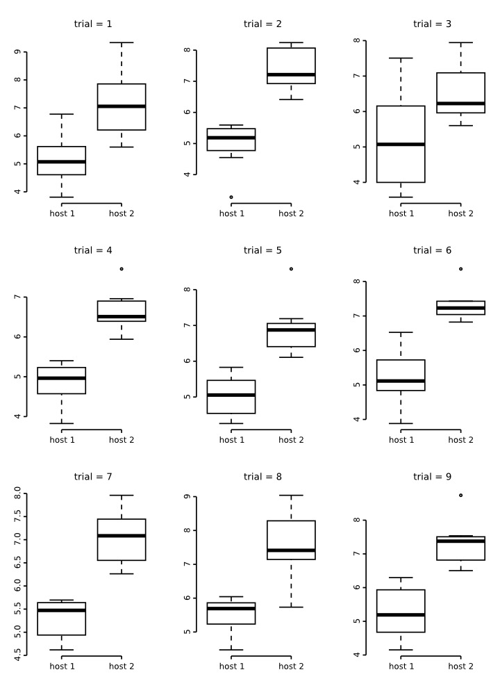
Figure 9. Box plot for 9 trials of sample size = 7 from random samples withdrawn from the distributions in Figure 8.
A close inspections of these box plots reveal that in 2/3 of them the ranges did not overlap despite their original distribution. Also, note that in all of them, the plots are not symmetric, suggesting that the distribution of the data is not normal. All of these attributes are artefacts of a small sample size. Consider that that is the same sample size used for the groups of the plots we generated for testes number and total length above!
Now, look at the behavior of these plots as sample size increases:

Figure 10. Box plot for 9 trials of sample sizes (N) varying from 10 to 10000 from random samples withdrawn from the distributions in Figure 8.
As can be shown in these box plots above, as the sample sizes increases the more obvious is the overlap between these two distributions. One this to notice as well as that after 200 samples, all plots become symmetric – reflecting the properties of the population distribution, that is, normality. Finally, observe that even withdrawing random numbers from the distribution, the box plots still recognizing some of them as outliers. That illustrate that even if box plots regard some values as outliers they can still be par of your distribution.
Literature cited
Fisher, R.A. 1918. The correlation between relatives on the supposition of Mendelian inheritance. Transactions of the Royal Society of Edinburgh 52: 399–433.
Hurlbert S.H. 1984. Pseudoreplication and the design of ecological field experiments. Ecol Monogr, 54(2):187–211.
Klazema, A. 2014. Descriptive and Inferential Statistics: How to Analyze Your Data. https://www.udemy.com/blog/descriptive-and-inferential-statistics/ accessed on July, 2014.
Lane, D.M.; Scott, D.; Hebl, M.; Guerra, R.; Osherson, D and Ziemer, H. 2014. Introduction dto Statistics. Online Statistics Education: A Multimedia Course of Study (http://onlinestatbook.com/). Project Leader: David M. Lane, Rice University. Accessed on July, 2014.
Lazic, E.S. 2010. The problem of pseudoreplication in neuroscientific studies: is it affecting your analysis? BMC Neuroscience, 11:5.
Millar, R.B. & Anderson, M.R. 2004). Remedies for pseudoreplication. Fisheries Research, 70(2–3): 397–407.
Schank J.C. & Koehnle T.J. 2009. Pseudoreplication is a pseudoproblem. Journal of Comparative Psychology, 123(4):421–433.
Templenton, A.R. 2006. Population genetics and microevolutionay theory. Wiley & Sons, Inc.
Trochim, W.M.K. 2006. Descriptive Statistics. http://www.socialresearchmethods.net/kb/statdesc.php Accessed on July, 2014.
Tukey, J.W. 1977. Exploratory Data Analysis. Addison-Wesley.
Zuur, A.F., Ieno, A.N. & Elphick, C.S. 2010. A protocol for data exploration to avoid common statistical problems. Methods in Ecology and Evolution, 1:3–14.
User Tools
Page Tools
Site Tools
tech.txt · Last modified: 2019/03/29 13:34 by fplmarques
 Except where otherwise noted, content on this wiki is licensed under the following license: CC Attribution-Share Alike 4.0 International